My sister and I found a great lemon pound cake recipe and on December 24th, we went for it! We had all the ingredients but in the kitchen were several unmarked jars of white substances—flour, baking powder, baking soda, sugar, salt, powdered sugar….which is which?! Me being more data scientist than baker, the dilemma prompts me to think of a classification problem and not just any classification problem but a class imbalance classification problem. My sister and I not only need to know which ingredients to include but also how much to include of the unmarked jars.

Mult-Layer Perceptrons Theory:

Many machine learning algos can tackle this problem with ease but let’s assume we need high accuracy and decide to use a Artificial Neural Nets (ANN) algorithm. Furthermore, let’s focus on a feedforward, 3-layer multi-layer perceptrons (MLP):

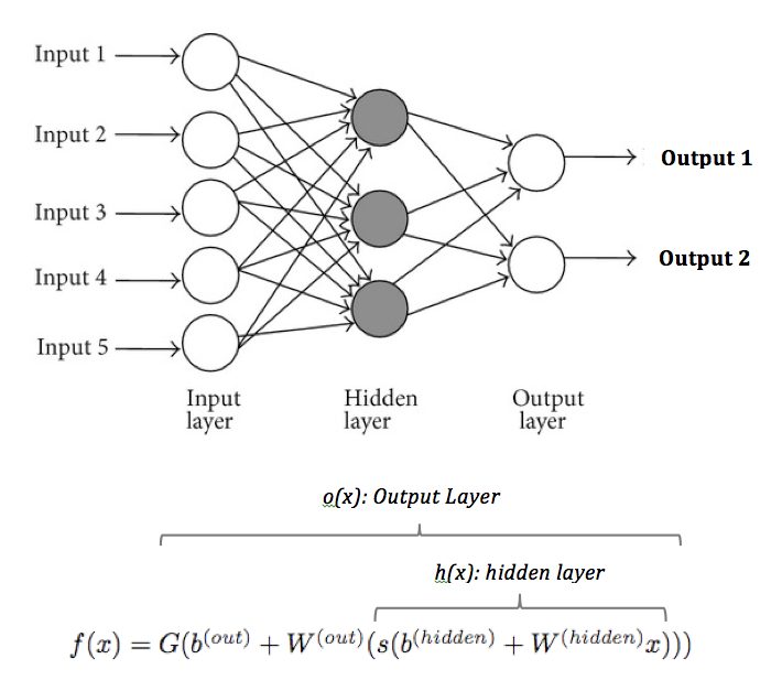
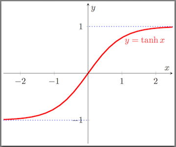
Key components of an MLP are the hidden layer(s) and fitting a non-linear function. If we didn’t include the hidden layer then the neural network would be a simple linear regression. Each hidden neuron takes inputs and weights them with a mean squared cost function—or another defined loss function—on the forward feed. Then, the output is put through an activation function s. Two most common activation functions for s are sigmoid (outputting 0 to 1) and tanh (outputting -1 to 1). Both tanh and sigmoid are scalar-to-scalar functions but we’ll utilize tanh because it creates a slightly larger range and tends to train faster. Comparison of the two functions is below:

Carrying from our first equation, the output from the hidden layer is then feed to the final output layer defined as:

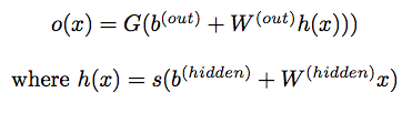
We’re looking for class-membership probabilities so G will be a softmax function.

Finally, we need to TRAIN our MLP! Here we’ll use Stochastic Gradient Descent (SGD) with minibatches. The set of parameters we’re learning are weights (W) and biases (b). We’ll obtain gradients from the backpropagation algorithm with each minibatch and then adjust the weights with the gradient learning rate. The biases will adjust according the loss function after the weights are adjusted.

SGD, Backprop, and Regularization are VERY important and, yes, I’m skimming over them right now because each topic requires a thorough explanation. Luckily, a lot of smart people have already written excellent tutorials about it here, here, and here.

So, let’s recap the MLP Algorithm:

1. Input layer feeds forward into hidden layer neurons
2. Each hidden layer neuron calculates an output with respect to the loss function
3. The hidden layer output is “squashed” by the activation function
4. The output layer receives the hidden layer output and calculates the final output with respect to the loss function
5. The final output is transformed to accommodate multi-class classification
6. Train the algorithm by backpropagation using SGD

Phew! There’s a reason why books are written on Neural Networks and Deep Learning. This only scratches the surface.

Note: DON’T FORGET to standardize the input data. Different magnitudes and distributions of input data could create bias and slow down the learning process. It isn’t strictly necessary to standardize the input data but it has several practical benefits. Perhaps more importantly, DO perform PCA and other techniques to decorrelate the inputs.

Correcting for Class Imbalance

Problems with class imbalance occur at two parts in the MLP: data sampling and cost function.

DATA SAMPLING

If we could just get evenly distributed classes then class imbalance wouldn’t exist! Oversampling, undersampling, or a little of both can be used to even out class imbalance. Of course, BE CAREFUL not to throw away data that could add important information to your model. Also, check feature variances before and after the resampling. If the sample distributions & variances match the population distributions & variances then you’re ready to give the new sample a try.

Another option is to reclassify the classes to binary. In the lemon pound cake example, let’s see if we can correctly classify sugar & salt (crystals) vs flour & baking soda (powder). Then, we can run an additional classifier for each sub-class to form a classifier chain ensemble. This method adds to the complexity of the model and, in general, is a long shot to improve accuracy. Still, it’s an option that might work beautifully if the data splits easily.

REDEFINE COST FUNCTION

The heart of the class imbalance lies with the cost function. In our MLP, we selected a mean squared cost function. In order to compensate for imbalanced classes, we want to penalize an error in less frequent classes more than frequent classes. In our new cost function, we’ll penalize each class by the inverse of the class share.

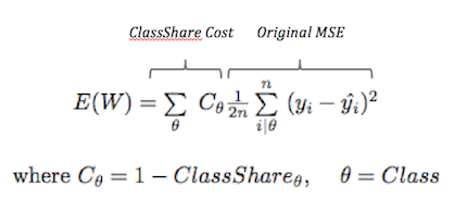
For example, if class x is .2 and class y is .8 of the total class share, then costx = .8 and costy = .2. This will “give more say” to the little guy in adjusting the error. Our new cost function is then used to calculate the gradient for backpropagation tuning.

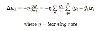
Beautiful! That’s are gradient we’ll use to tune our MLP and attempt to rebalance our imbalance by weighting the errors according to the class share. Our adjusted model has compensated, as best it can, for class imbalance. Hopefully, with a lot of careful consideration, the model will turn out something like this.

Note: Not every is a fan of Lemon Pound Cake examples. So, I actually came across this problem while working with HDMA data from the Consumer Financial Protection Bureau. The data consists of mortgage approvals and mortgage selling in the secondary markets. The purpose is to keep banks accountable of possible predator or improper loan approval/denials. The data engineering from the HDMA API can be found here and the full ML script in Jupyter notebook can be found here. I’ll be making additional updates to the ML script soon……